低通濾波器實驗代碼，這是參考別人網(wǎng)上的代碼，所以自己也分享一下，共同進步

# -*- coding: utf-8 -*-import numpy as npfrom scipy.signal import butter, lfilter, freqzimport matplotlib.pyplot as pltdef butter_lowpass(cutoff, fs, order=5): nyq = 0.5 * fs normal_cutoff = cutoff / nyq b, a = butter(order, normal_cutoff, btype=’low’, analog=False) return b, adef butter_lowpass_filter(data, cutoff, fs, order=5): b, a = butter_lowpass(cutoff, fs, order=order) y = lfilter(b, a, data) return y # Filter requirements.order = 6fs = 30.0 # sample rate, Hzcutoff = 3.667 # desired cutoff frequency of the filter, Hz # Get the filter coefficients so we can check its frequency response.b, a = butter_lowpass(cutoff, fs, order) # Plot the frequency response.w, h = freqz(b, a, worN=800)plt.subplot(2, 1, 1)plt.plot(0.5*fs*w/np.pi, np.abs(h), ’b’)plt.plot(cutoff, 0.5*np.sqrt(2), ’ko’)plt.axvline(cutoff, color=’k’)plt.xlim(0, 0.5*fs)plt.title('Lowpass Filter Frequency Response')plt.xlabel(’Frequency [Hz]’)plt.grid() # Demonstrate the use of the filter. # First make some data to be filtered.T = 5.0 # secondsn = int(T * fs) # total number of samplest = np.linspace(0, T, n, endpoint=False) # 'Noisy' data. We want to recover the 1.2 Hz signal from this.data = np.sin(1.2*2*np.pi*t) + 1.5*np.cos(9*2*np.pi*t) + 0.5*np.sin(12.0*2*np.pi*t) # Filter the data, and plot both the original and filtered signals.y = butter_lowpass_filter(data, cutoff, fs, order)plt.subplot(2, 1, 2)plt.plot(t, data, ’b-’, label=’data’)plt.plot(t, y, ’g-’, linewidth=2, label=’filtered data’)plt.xlabel(’Time [sec]’)plt.grid()plt.legend()plt.subplots_adjust(hspace=0.35)plt.show()

實際代碼，沒有整理，可以讀取txt文本文件，然后進行低通濾波，并將濾波前后的波形和FFT變換都顯示出來

# -*- coding: utf-8 -*-import numpy as npfrom scipy.signal import butter, lfilter, freqzimport matplotlib.pyplot as pltimport osdef butter_lowpass(cutoff, fs, order=5): nyq = 0.5 * fs normal_cutoff = cutoff / nyq b, a = butter(order, normal_cutoff, btype=’low’, analog=False) return b, adef butter_lowpass_filter(data, cutoff, fs, order=5): b, a = butter_lowpass(cutoff, fs, order=order) y = lfilter(b, a, data) return y # Filter requirements.order = 5fs = 100000.0 # sample rate, Hzcutoff = 1000 # desired cutoff frequency of the filter, Hz # Get the filter coefficients so we can check its frequency response.# b, a = butter_lowpass(cutoff, fs, order) # Plot the frequency response.# w, h = freqz(b, a, worN=1000)# plt.subplot(3, 1, 1)# plt.plot(0.5*fs*w/np.pi, np.abs(h), ’b’)# plt.plot(cutoff, 0.5*np.sqrt(2), ’ko’)# plt.axvline(cutoff, color=’k’)# plt.xlim(0, 1000)# plt.title('Lowpass Filter Frequency Response')# plt.xlabel(’Frequency [Hz]’)# plt.grid() # Demonstrate the use of the filter. # First make some data to be filtered.# T = 5.0 # seconds# n = int(T * fs) # total number of samples# t = np.linspace(0, T, n, endpoint=False) # 'Noisy' data. We want to recover the 1.2 Hz signal from this.# # data = np.sin(1.2*2*np.pi*t) + 1.5*np.cos(9*2*np.pi*t) + 0.5*np.sin(12.0*2*np.pi*t) # Filter the data, and plot both the original and filtered signals.path = '*****'for file in os.listdir(path): if file.endswith('txt'): data=[] filePath = os.path.join(path, file) with open(filePath, ’r’) as f: lines = f.readlines()[8:] for line in lines: # print(line) data.append(float(line)*100) # print(len(data)) t1=[i*10 for i in range(len(data))] plt.subplot(231) # plt.plot(range(len(data)), data) plt.plot(t1, data, linewidth=2,label=’original data’) # plt.title(’ori wave’, fontsize=10, color=’#F08080’) plt.xlabel(’Time [us]’) plt.legend() # filter_data = data[30000:35000] # filter_data=data[60000:80000] # filter_data2=data[60000:80000] # filter_data = data[80000:100000] # filter_data = data[100000:120000] filter_data = data[120000:140000] filter_data2=filter_data t2=[i*10 for i in range(len(filter_data))] plt.subplot(232) plt.plot(t2, filter_data, linewidth=2,label=’cut off wave before filter’) plt.xlabel(’Time [us]’) plt.legend() # plt.title(’cut off wave’, fontsize=10, color=’#F08080’) # filter_data=zip(range(1,len(data),int(fs/len(data))),data) # print(filter_data) n1 = len(filter_data) Yamp1 = abs(np.fft.fft(filter_data) / (n1 / 2)) Yamp1 = Yamp1[range(len(Yamp1) // 2)] # x_axis=range(0,n//2,int(fs/len # 計算最大賦值點頻率 max1 = np.max(Yamp1) max1_index = np.where(Yamp1 == max1) if (len(max1_index[0]) == 2): print((max1_index[0][0] )* fs / n1, (max1_index[0][1]) * fs / n1) else: Y_second = Yamp1 Y_second = np.sort(Y_second) print(np.where(Yamp1 == max1)[0] * fs / n1, (np.where(Yamp1 == Y_second[-2])[0]) * fs / n1) N1 = len(Yamp1) # print(N1) x_axis1 = [i * fs / n1 for i in range(N1)] plt.subplot(233) plt.plot(x_axis1[:300], Yamp1[:300], linewidth=2,label=’FFT data’) plt.xlabel(’Frequence [Hz]’) # plt.title(’FFT’, fontsize=10, color=’#F08080’) plt.legend() # plt.savefig(filePath.replace('txt', 'png')) # plt.close() # plt.show() Y = butter_lowpass_filter(filter_data2, cutoff, fs, order) n3 = len(Y) t3 = [i * 10 for i in range(n3)] plt.subplot(235) plt.plot(t3, Y, linewidth=2, label=’cut off wave after filter’) plt.xlabel(’Time [us]’) plt.legend() Yamp2 = abs(np.fft.fft(Y) / (n3 / 2)) Yamp2 = Yamp2[range(len(Yamp2) // 2)] # x_axis = range(0, n // 2, int(fs / len(Yamp))) max2 = np.max(Yamp2) max2_index = np.where(Yamp2 == max2) if (len(max2_index[0]) == 2): print(max2, max2_index[0][0] * fs / n3, max2_index[0][1] * fs / n3) else: Y_second2 = Yamp2 Y_second2 = np.sort(Y_second2) print((np.where(Yamp2 == max2)[0]) * fs / n3, (np.where(Yamp2 == Y_second2[-2])[0]) * fs / n3) N2=len(Yamp2) # print(N2) x_axis2 = [i * fs / n3 for i in range(N2)] plt.subplot(236) plt.plot(x_axis2[:300], Yamp2[:300],linewidth=2, label=’FFT data after filter’) plt.xlabel(’Frequence [Hz]’) # plt.title(’FFT after low_filter’, fontsize=10, color=’#F08080’) plt.legend() # plt.show() plt.savefig(filePath.replace('txt', 'png')) plt.close() print(’*’*50) # plt.subplot(3, 1, 2) # plt.plot(range(len(data)), data, ’b-’, linewidth=2,label=’original data’) # plt.grid() # plt.legend() # # plt.subplot(3, 1, 3) # plt.plot(range(len(y)), y, ’g-’, linewidth=2, label=’filtered data’) # plt.xlabel(’Time’) # plt.grid() # plt.legend() # plt.subplots_adjust(hspace=0.35) # plt.show() ’’’ # Y_fft = Y[60000:80000] Y_fft = Y # Y_fft = Y[80000:100000] # Y_fft = Y[100000:120000] # Y_fft = Y[120000:140000] n = len(Y_fft) Yamp = np.fft.fft(Y_fft)/(n/2) Yamp = Yamp[range(len(Yamp)//2)] max = np.max(Yamp) # print(max, np.where(Yamp == max)) Y_second = Yamp Y_second=np.sort(Y_second) print(float(np.where(Yamp == max)[0])* fs / len(Yamp),float(np.where(Yamp==Y_second[-2])[0])* fs / len(Yamp)) # print(float(np.where(Yamp == max)[0]) * fs / len(Yamp)) ’’’

補充拓展：淺談opencv的理想低通濾波器和巴特沃斯低通濾波器

低通濾波器

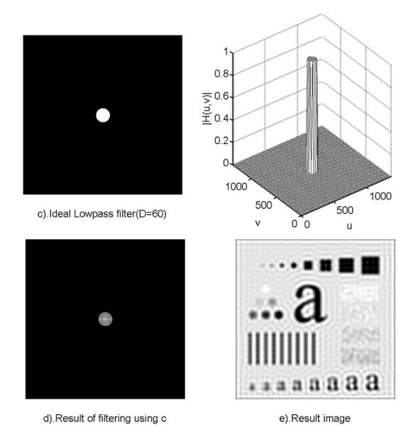
1.理想的低通濾波器

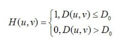
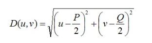
其中，D0表示通帶的半徑。D(u,v)的計算方式也就是兩點間的距離，很簡單就能得到。

使用低通濾波器所得到的結果如下所示。低通濾波器濾除了高頻成分，所以使得圖像模糊。由于理想低通濾波器的過度特性過于急峻，所以會產(chǎn)生了振鈴現(xiàn)象。

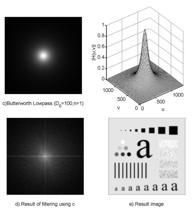
2.巴特沃斯低通濾波器

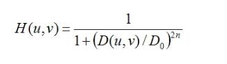
同樣的，D0表示通帶的半徑，n表示的是巴特沃斯濾波器的次數(shù)。隨著次數(shù)的增加，振鈴現(xiàn)象會越來越明顯。

void ideal_Low_Pass_Filter(Mat src){Mat img;cvtColor(src, img, CV_BGR2GRAY);imshow('img',img);//調(diào)整圖像加速傅里葉變換int M = getOptimalDFTSize(img.rows);int N = getOptimalDFTSize(img.cols);Mat padded;copyMakeBorder(img, padded, 0, M - img.rows, 0, N - img.cols, BORDER_CONSTANT, Scalar::all(0));//記錄傅里葉變換的實部和虛部Mat planes[] = { Mat_<float>(padded), Mat::zeros(padded.size(), CV_32F) };Mat complexImg;merge(planes, 2, complexImg);//進行傅里葉變換dft(complexImg, complexImg);//獲取圖像Mat mag = complexImg;mag = mag(Rect(0, 0, mag.cols & -2, mag.rows & -2));//這里為什么&上-2具體查看opencv文檔//其實是為了把行和列變成偶數(shù) -2的二進制是11111111.......10 最后一位是0//獲取中心點坐標int cx = mag.cols / 2;int cy = mag.rows / 2;//調(diào)整頻域Mat tmp;Mat q0(mag, Rect(0, 0, cx, cy));Mat q1(mag, Rect(cx, 0, cx, cy));Mat q2(mag, Rect(0, cy, cx, cy));Mat q3(mag, Rect(cx, cy, cx, cy)); q0.copyTo(tmp);q3.copyTo(q0);tmp.copyTo(q3); q1.copyTo(tmp);q2.copyTo(q1);tmp.copyTo(q2);//Do為自己設定的閥值具體看公式double D0 = 60;//處理按公式保留中心部分for (int y = 0; y < mag.rows; y++){double* data = mag.ptr<double>(y);for (int x = 0; x < mag.cols; x++){double d = sqrt(pow((y - cy),2) + pow((x - cx),2));if (d <= D0){}else{data[x] = 0;}}}//再調(diào)整頻域q0.copyTo(tmp);q3.copyTo(q0);tmp.copyTo(q3);q1.copyTo(tmp);q2.copyTo(q1);tmp.copyTo(q2);//逆變換Mat invDFT, invDFTcvt;idft(mag, invDFT, DFT_SCALE | DFT_REAL_OUTPUT); // Applying IDFTinvDFT.convertTo(invDFTcvt, CV_8U);imshow('理想低通濾波器', invDFTcvt);} void Butterworth_Low_Paass_Filter(Mat src){int n = 1;//表示巴特沃斯濾波器的次數(shù)//H = 1 / (1+(D/D0)^2n)Mat img;cvtColor(src, img, CV_BGR2GRAY);imshow('img', img);//調(diào)整圖像加速傅里葉變換int M = getOptimalDFTSize(img.rows);int N = getOptimalDFTSize(img.cols);Mat padded;copyMakeBorder(img, padded, 0, M - img.rows, 0, N - img.cols, BORDER_CONSTANT, Scalar::all(0)); Mat planes[] = { Mat_<float>(padded), Mat::zeros(padded.size(), CV_32F) };Mat complexImg;merge(planes, 2, complexImg); dft(complexImg, complexImg); Mat mag = complexImg;mag = mag(Rect(0, 0, mag.cols & -2, mag.rows & -2)); int cx = mag.cols / 2;int cy = mag.rows / 2; Mat tmp;Mat q0(mag, Rect(0, 0, cx, cy));Mat q1(mag, Rect(cx, 0, cx, cy));Mat q2(mag, Rect(0, cy, cx, cy));Mat q3(mag, Rect(cx, cy, cx, cy)); q0.copyTo(tmp);q3.copyTo(q0);tmp.copyTo(q3); q1.copyTo(tmp);q2.copyTo(q1);tmp.copyTo(q2); double D0 = 100; for (int y = 0; y < mag.rows; y++){double* data = mag.ptr<double>(y);for (int x = 0; x < mag.cols; x++){//cout << data[x] << endl;double d = sqrt(pow((y - cy), 2) + pow((x - cx), 2));//cout << d << endl;double h = 1.0 / (1 + pow(d / D0, 2 * n));if (h <= 0.5){data[x] = 0;}else{//data[x] = data[x]*0.5;//cout << h << endl;}//cout << data[x] << endl;}}q0.copyTo(tmp);q3.copyTo(q0);tmp.copyTo(q3);q1.copyTo(tmp);q2.copyTo(q1);tmp.copyTo(q2);//逆變換Mat invDFT, invDFTcvt;idft(complexImg, invDFT, DFT_SCALE | DFT_REAL_OUTPUT); // Applying IDFTinvDFT.convertTo(invDFTcvt, CV_8U);imshow('巴特沃斯低通濾波器', invDFTcvt);}

以上這篇python實現(xiàn)低通濾波器代碼就是小編分享給大家的全部內(nèi)容了，希望能給大家一個參考，也希望大家多多支持好吧啦網(wǎng)。